Multiple regression analysis is used to examine the relationship between one numerical variable, called a criterion, and a set of other variables, called predictors. In addition, multiple regression analysis is used to investigate the correlation between two variables after controlling another covariate.
To illustrate, consider a researcher who wants to know whether or not the number of jars of Chicken Tonite you consume--the dependent variable or criterion--relates to frequency of psychotic behaviours, frequency of crossing roads, and age--the independent variables or predictors.
Multiple regression serves two functions. First, this technique yields an equation that predicts the dependent variable or criterion from the various independent variables or predictors. This function, however, is seldom utilised in psychology. Second, and more importantly, this technique identifies the independent variables that relate to the dependent variable, after controlling the other variables. For instance, this procedure can determine the relationship between Chicken Tonite and crossing roads in individuals who are equivalent on psychotic behaviours, age, and so on.
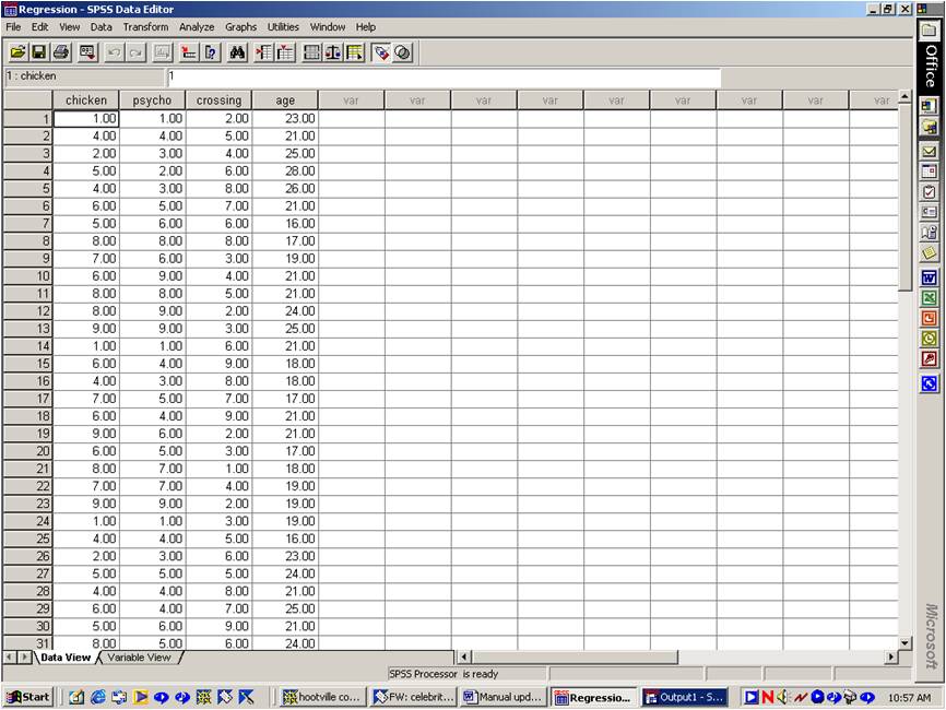
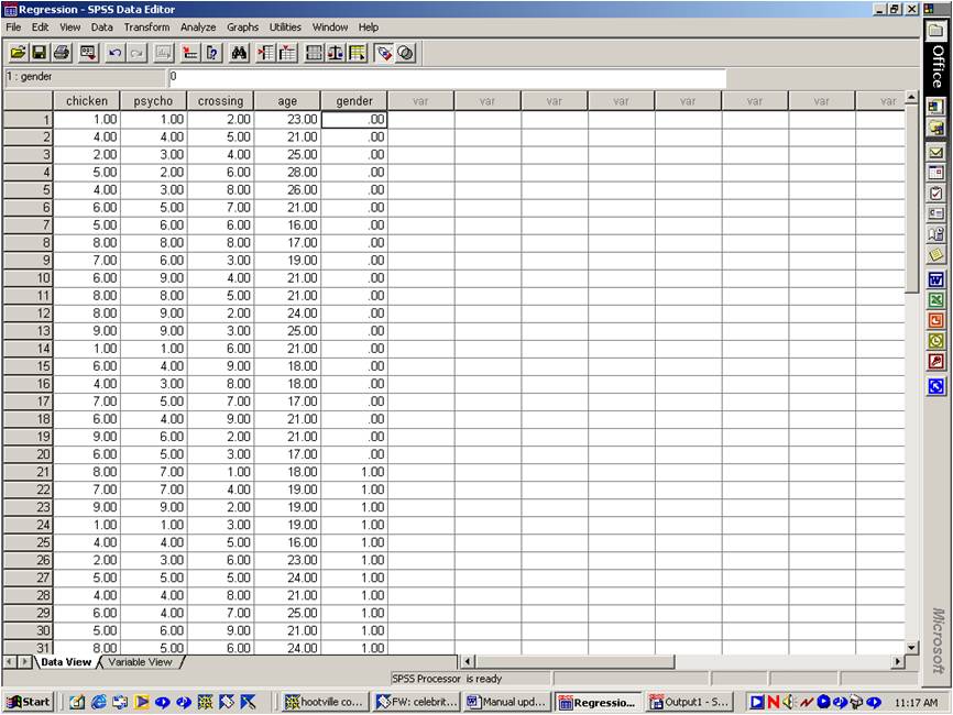
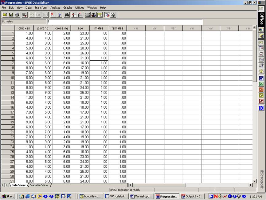
To demonstrate multiple regression, you should first access SPSS and create a data file that resembles the following.
To subject these data to multiple regression:

Regression assumes the dependent or criterion variable can be predicted from the independent or predictor variables using an equation. The equation is assumed to resemble the following formula:
Dependent variable = B0 + B1 x iv1 + B2 x iv2 + B3 x iv3 ...
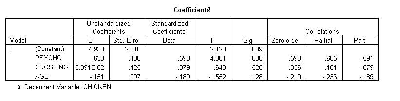
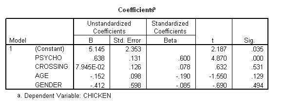
The B values denote numbers, such as 3.6. Using some special formula, multiple regression then estimates these B values. These B values are then reported in the column labelled B. Locate this column in the previous outcome. These B values can then be used to specify the equation. Note that 8.09E-02 denotes 8.09 x 10⁻², which equals 0.0809;; that is, the decimal place is moved two places to the left. In this case, the equation is:
Chicken = 4.933 + 0.630 x Psycho + 0.081 x Crossing--0.151 x Age
This equation can be used to predict the dependent variable from the independent variables. To illustrate, suppose that a person scored 2 for "Psycho", 8 for "Crossing", and 10 for "Age". Now, enter these values into the equation. This process yields a 5.33. That is, we predict this participant will score 5.33 on the dependent variable or criterion "Chicken".
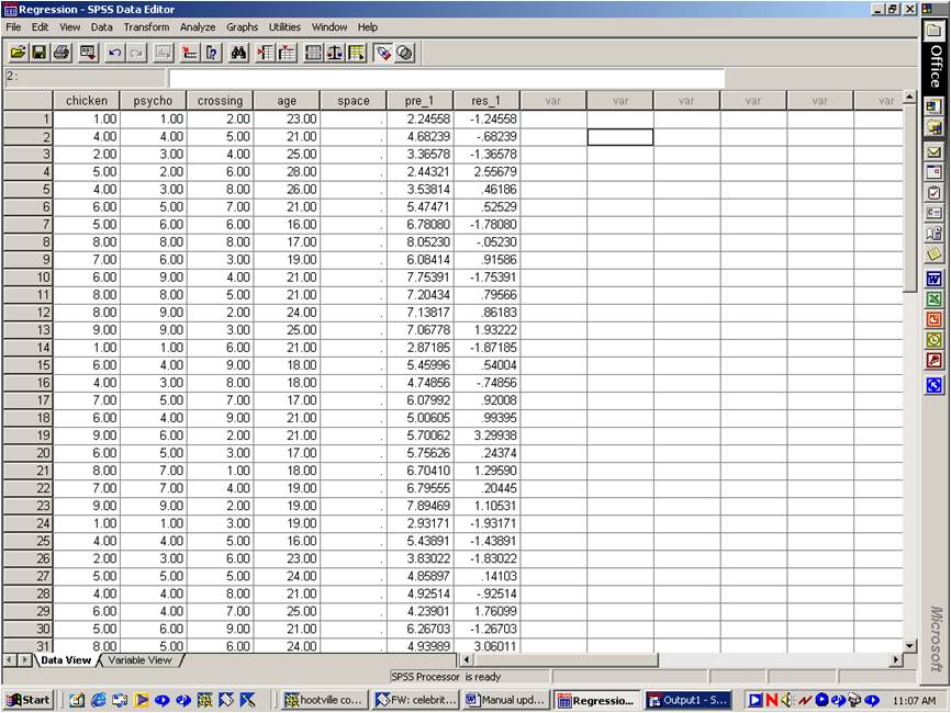
This equation is regarded as accurate if the residuals are minimal. To illustrate the concept of residuals:
Indeed, SPSS can be utilised to compute the predicted dependent variable and the residuals associated with each individual.
Furthermore, a statistic called Multiple R represents the correlation between the predicted dependent variable and the actual dependent variable, a value that ideally approaches 1. SPSS also provides the square of this value. This value, R squared, represents the percentage of variance in the dependent variable that is explained by the independent variables. To appreciate this concept:
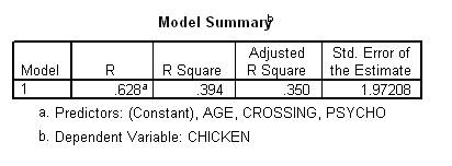
The value of R squared that was derived from the sample tends to exceed the value of R squared in the population. For instance:
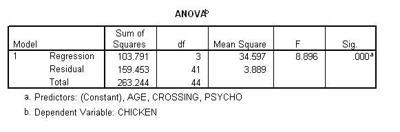
The F value and also the corresponding significance or p value reflects whether or not R squared significantly differs from zero. When this significance value is less than alpha or 0.05, the R squared value significantly differs from 0. That is, the dependent variable is significantly related to the independent variables. When this significance value exceeds alpha or 0.05, the R squared value does not significantly differ from 0. In other words, the dependent variable is not significantly related to the independent variables. This F and p value is presented below.
Multiple regression can also ascertain which of the independent variables relate to the dependent variable. You might believe that Pearson's correlation can answer this question. For example, suppose the correlation between "Psycho" and "Chicken" was significant. You might then conclude that "Psycho" significantly relates to "Chicken. However:
To resolve this issue, examine the column labelled "Sig" in the coefficients table, which provides the p values. In particular:
In other words, some element of Psycho that is unrelated to Crossing or Age must be correlated with Chicken. To appreciate this claim, you should recognise that:
The p value associated with "Crossing" exceeds alpha or 0.05. Hence, the corresponding B value does not differ significantly from 0. We thus conclude that "Crossing does not relate to Chicken after controlling for Psycho and Age".
To reiterate, the B value associated with "Psycho" significantly differed from 0. The next step is to interpret the sign of this B value in the coefficients table, which is presented again below.
In some instance, a significant B value may be negative. In this situation,
The final step is to interpret the part correlations--often called semi-partial correlations. Specifically:
To compute the part correlation between two variables Y and A, after controlling another variable B, the following formula would be utilised.
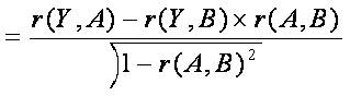
This formula is merely presented to demonstrate the part correlation is elevated if:
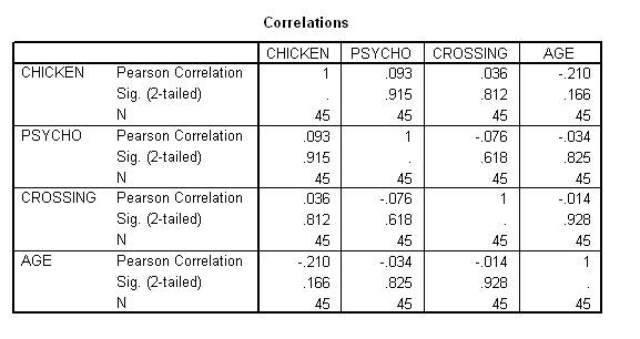
Consider the following table that reveals the correlation between each pair of measures. In this instance, Psycho does not seem to correlate significantly with Chicken.
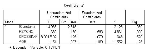
In contrast, consider the following table, which provides the output that emerged from multiple regression. In this instance, Psycho does relate to Chicken. The impact of Psycho on Chicken emerged only after the other predictors were controlled. Researchers utilise the following terminology to describe this instance. They claim that Crossing or Age had suppressed the relationship between Psycho and Chicken. This relationship emerged only after these suppressor variables were controlled.
In short, a predictor might be unrelated to the criterion according to a correlation matrix but related to the criterion according to a multiple regression. This situation can arise if the relationship between two of the variables is negative, but the relationship between all the other variables is positive. In addition, this situation can arise if the relationship between all the variables is negative. To illustrate, suppose the relationships between Chicken, Psycho, and Crossing correspond to the following model.
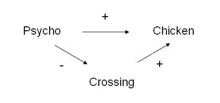
This model reveals that Psycho influences Chicken via two pathways. According to the top pathway, Psycho directly promotes Chicken. According to the bottom pathway, Psycho indirectly reduces Chicken. That is, Psycho impedes Crossing and thus Chicken. Therefore,
In short, according to this model, the correlation between Psycho and Chicken should not be significant. In addition, when a multiple regression is conducted, and Crossing is controlled, Psycho should be positively related to Chicken. The previous correlation matrix and regression coefficients thus corroborate this model.
Sometimes, several independent variables are significant. You may thus want to identify the independent variable that bestows the greatest impact on the dependent variable. In this endeavour, you may be tempted to utilise the B values. However, the magnitude of these B values depends on both:
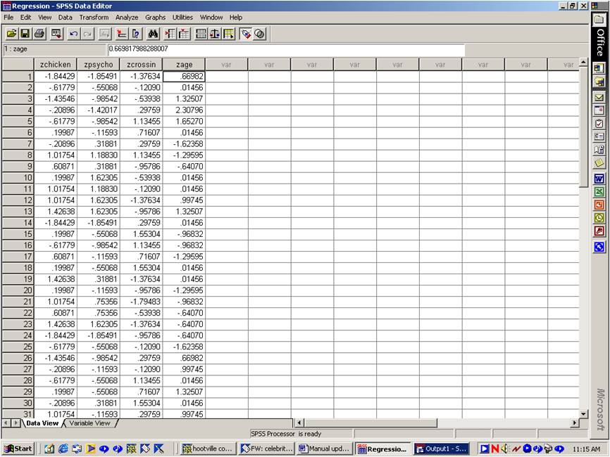
Therefore, these B values do not represent importance only. To overcome this problem, SPSS converts all of the raw data into z scores, as depicted below, and recomputes the B values. These z scores--which are presented below--are computed by deducting the mean from the original values and then dividing by the standard deviation. Accordingly, the mean of these z scores is zero and the standard deviation is 1. These B values--which are called unstandardised--are displayed in the column labelled Beta. Because these B values were derived from z scores, all the independent variables yield the same variance. Hence, the magnitude of these B values represents the importance of each independent variable. Roughly speaking, higher Beta values tend to reflect more important independent variables.
In general, the independent variables need to be numerical. Fortunately, multiple regression can also exploit dichotomous independent variables--that is, independent variables that entail two categories. Gender is one example. To this end,
To interpret this added predictor:
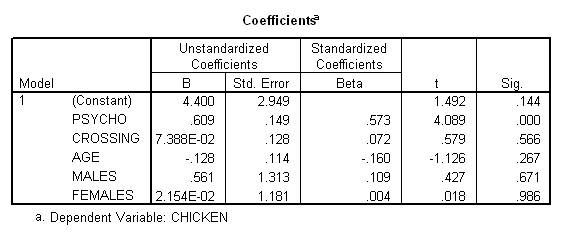
Dummy coding can be extended to independent variables that entail more than two categories. For example, suppose the first five participants were actually hermaphrodites. To represent this situation, you first need to discard the column labelled "Gender". Add two new columns--"Males" and "Female". In the "Male" column, 1s represent males and 0s represent the others. In the "Female" column, 1s represent females and 0s represent others. An example is presented below.
You might be tempted to include a column labelled "hermaphrodites"& this step would yield a problem called singularity. Specifically, this column would simply equal 1 minus the two other columns, which represents an extreme form of an issue called multi-colinearity. To interpret the outcome of these analyses:
Sometimes, you would prefer to ascertain whether or not each category differs from the average participant. In this instance, you might be interested in whether or not males and females differ from the average participant. In other words, you might not be interested in whether or not males and females differ from hermaphrodites. To fulfil this purpose, you need to adjust the dummy variables. Specifically, replace the 0s with -1 for participants who pertain to the reference category. That is, substitute the 0s with -1 for each hermaphrodite. The following output will then emerge.
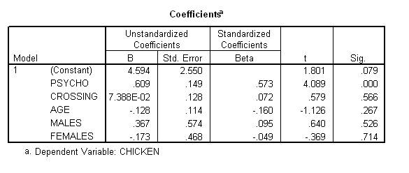
According to this output, neither males nor females differ significantly from the average participant. Whether or not hermaphrodites differ significantly from the average participant cannot be determined from these data. Researchers could repeat the analysis and designate another gender, such as males, as the reference category.
Consider a researcher who has measured 50 predictors of chicken tonight--perhaps five personality variables, eight family variables, six economic variables, and so forth. Unless the sample size is very large, the researcher cannot include all 50 predictors in the same regression analysis. How many regression analyses should this researcher conduct? Perhaps the researcher could:
This strategy seems reasonable. Nevertheless, to decide which strategy is optimal, the researcher should reflect upon the benefits of examining several predictors in the same regression analysis. To demonstrate, suppose five personality variables are subjected to the same regression analysis. Thus, by definition, each personality variable is examined after controlling the other personality variables. The question, therefore, becomes what are the benefits of controlling other variables. Four benefits of controlling variables can be differentiated:
In this instance, the researcher most likely decided to:
In short, to decide which predictors to include in the multiple regression analysis, you should consider whether you want to purify measures, control spurious factors, examine mediators, or increase power. Nevertheless, in practice, researchers tend to include variables that correspond to a similar category in the same analysis. They also control demographics that seem to correlate with both the dependent and independent variables.
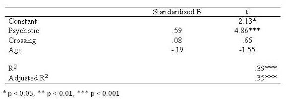
A multiple regression analysis was used to examine whether psychotic behaviour, crossing roads, and age was related to the number of jars of Chicken Tonite that individuals consume. The B and t values that emerged are presented in Table 1. Table 1 reveals that psychoticism increases the volume of Chicken Tonite that individuals consume after controlling age and the frequency with which they crossed roads. None of the other predictors achieved significance.
Table 1. Output of the regression that related consumption of Chicken Tonite to psychoticism, crossing roads, and age
Last Update: 7/7/2016