ANCOVAs are utilised to compare groups, such as males and females, on one numerical variable, such as IQ, if you also want to control other numerical variables.
Consider a researcher who claims the tortellini at Monash University reduces weight, primarily because individuals feel a desperate urge to scurry repeatedly to the toilet. The researcher records the weight and height of individuals who regularly consume the tortellini as well as a control group who shun this dish. An extract of the findings are provided below. The bottom row provides the average weight of each group.
| Consumes tortellini | Shuns tortellini | ||
|---|---|---|---|
| Weight (kg) | Height (cm) | Weight (kg) | Height (cm) |
| 85 | 183 | 80 | 187 |
| 62 | 159 | 58 | 159 |
| 71 | 169 | 61 | 165 |
| 89 | 184 | 69 | 171 |
| . | . | . | . |
| . | . | . | . |
| 89 | 174 | 73 | 178 |
| Average = 74.1 | | Average = 67.9 | |
In this example, the researcher might want to control height. That is, the researcher might need to ascertain whether tortellini consumption still influences weight even when height is controlled--that is, even in participants whose height is equivalent. To control this variable, the researcher could potentially estimate the weight each individual would have reached had their height been average. For example:
| Consumes tortellini | Shuns tortellini | ||
|---|---|---|---|
| Real weight (kg) | Adjusted weight (kg) | Real weight (kg) | Adjusted weight (kg) |
| 85 | 76 | 80 | 66 |
| 62 | 70 | 58 | 69 |
| 71 | 70 | 61 | 67 |
| 89 | 78 | 69 | 70 |
| . | . | . | . |
| . | . | . | . |
| 89 | 88 | 73 | 68 |
| Average = 74.1 | Average = 74.07 | Average = 67.9 | Average = 67.88 |
A t-test or ANOVA could then be applied to these adjusted weights. In short, the researcher often needs to estimate the values on some measure that individuals would have reached had they been average on another variable, sometimes called the covariate. Of course, this process seems cumbersome and imprecise. Fortunately, SPSS undertakes a technique that undertakes this entire process systematically and rapidly. This technique is called an analysis of covariance or ANCOVA.
In essence, SPSS undertakes three processes. First, SPSS estimates the values on the dependent measure that individuals would have reached had they been average on the covariate. Second, SPSS adjusts the df associated with MS error. In particular, the number of covariates is deducted from this df value--which is merely a technical adjustment. Finally, an ANOVA is applied to the adjusted scores. This set of processes may seem complex.
However, in practice, the user merely needs to complete a few simple steps. If possible, conduct these steps as you read the following section.
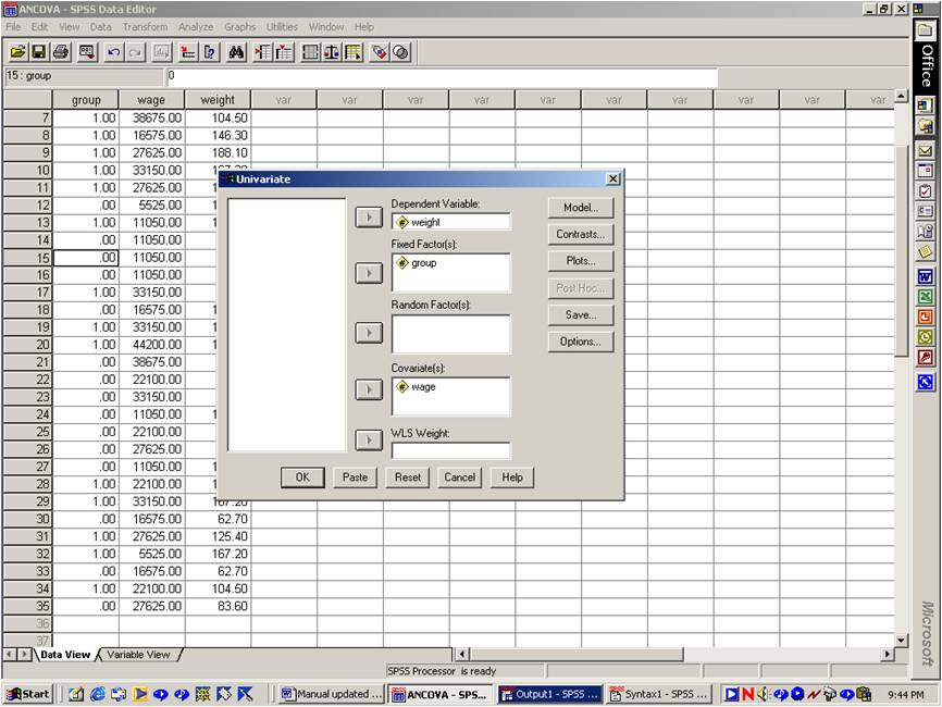
This covariate can be conceptualized as merely another factor. However, unlike other factors, this covariate is numerical rather than categorical. Also, SPSS does not examine the interaction between this covariate and other factors unless specified otherwise.
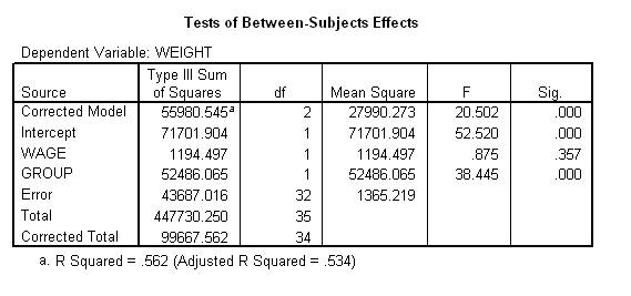
This process yields the following table. Recall the researcher is merely interested in whether or not weight varies across group. Hence, they should locate the row that pertains to this factor, and then identify the p value, which in this instance approximates .000. This p value is less than 0.05 or alpha and thus indicates that weight differs between the two groups, after controlling wage. As an aside:
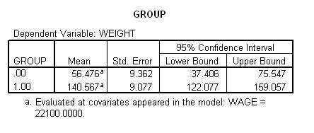
To determine which group tends to yield more weight, after controlling wage, the researcher should consult the following table. This table presents the mean that would have emerged from each group had the individuals been average on the covariate. In this instance, the mean is higher in the individuals who consume tortellini. Thus, tortellini increases weight, even after controlling wage.
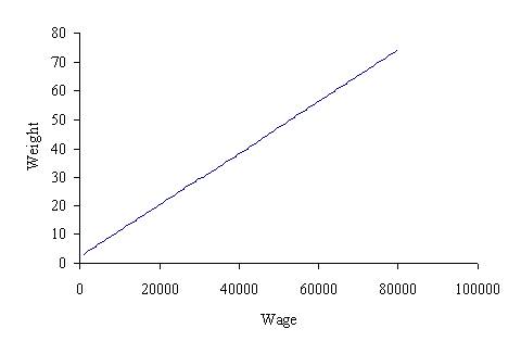
Thus far, the discussion has assumed the measures, such as weight, are adjusted haphazardly. That is, this discussion assumed the computer merely estimates the score the individuals would have reached had they been average on the covariates. In practice, a systematic technique is utilised to adjust these measures. Essentially, to adjust the dependent measure:
This relationship is depicted below.
In some instances, researchers could include several covariates. For example, the researcher could include wage, height, IQ, personality, and many other covariates in the design. The question, then, becomes which of these covariates should be included. The following principles need to be considered:
Indeed, the inclusion of extraneous variables can actually reduce power. That is, each covariate reduces the df values associated with the error term. This reduction of the df increases MS error and thus diminishes F. This reduction in F raises the p value, and thus impedes the likelihood of significant effects. In a nutshell, irrelevant covariates should be excluded as a means to increase power.
To reiterate, SPSS adjusts the dependent measure to predict the score that would have been observed if the participant was average on the covariates. To ascertain the magnitude of this adjustment, SPSS examines the relationship between the dependent measure and covariate. This process assumes the relationship between the dependent measure and covariate is the same in each group. This assumption, however, is often violated. For example, in individuals who consume tortellini, the relationship between the dependent measure and covariate could conform to the following equation:
In contrast, in individuals who shun tortellini, the relationship between the dependent measure and covariate could conform to a different equation, such as:
That is, weight might be more related to wage in one group compared to the other group. When the relationship between the dependent measure and covariate differs between the groups, the adjustment that SPSS imposes is not appropriate. That is, SPSS utilises an equation that is not applicable to either group. Fortunately, this assumption can be readily assessed. Specifically, to assess this assumption:
If this p value is less than 0.05 or alpha, the relationship between the covariate and the dependent measure must differ between the groups. That is, the interaction indicates the effect of wage on weight depends on group. Hence, the assumption of homogenous regression must be violated. If the assumption is violated, moderated regression analysis should probably be conducted instead of ANCOVA.
An analysis of covariance or ANCOVA was undertaken to explore the effect of consuming tortellini on weight, after controlling height. The relationship between height and weight did not depend on tortellini consumption, F(1, 32) = 1.19, p >& .05, consistent with homogeneity of regression. Thus, the interaction between tortellini consumption and height was excluded from the ANCOVA. This ANCOVA revealed that tortellini consumption did indeed influence weight after controlling height, F(1, 32) = 38.44, p <& .001. Specifically, as indicated by the estimated marginal means, weight was elevated in individuals who consumed tortellini (X bar = 140.57, SE = 9.01) relative to control participants (X bar = 46.48, SE = 9.36).
Last Update: 7/7/2016