The software package called AMOS is used to undertake confirmatory factor analysis, structural equation modelling, and latent variable growth curve modelling (for more information, see Confirmatory factor analysis and Introduction to structural equation modeling). AMOS is now a component of SPSS. Nevertheless, AMOS is more difficult to use than other facets of SPSS. This document provides a tutorial to assist users of AMOS, but assumes some familiarity with exploratory factor analysis.
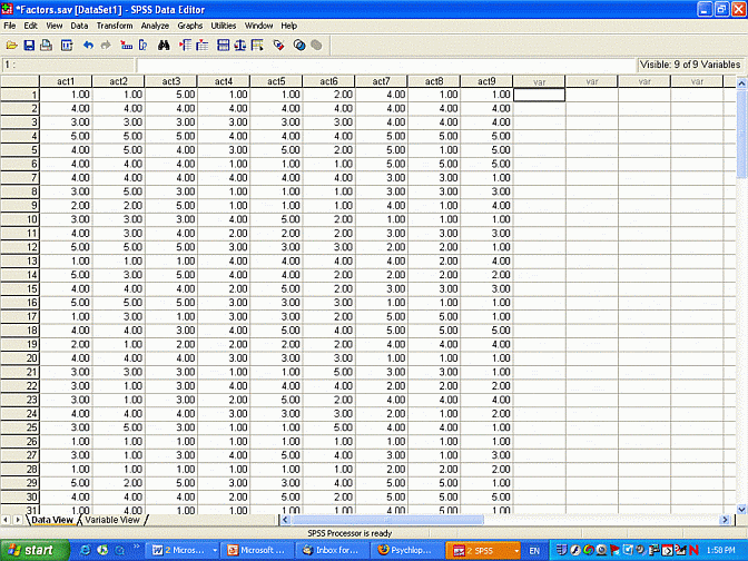
Suppose a researcher wants to ascertain the extent to which individuals engage in various peculiar behaviors. Individuals are asked to estimate the extent to which they undertake nine peculiar activities, on scale that ranges from one to five. Specifically, they are asked to estimate the extent to which they listen to Rolf Harris, discuss brands of nail clippers, enjoy statistics, store ear wax, examine gunk under toe nails, display their double jointed arms, ring people at 3.00 am, go home when it is their turn to shout drinks, and play music at maximum volume. An extract of the data is presented below.
Suppose that a previous analysis revealed that Acts 1 to 3 pertain to a factor called boring, Acts 4 to 6 pertain to a factor called vulgar, and Acts 7 to 9 pertain to a factor called insensitive. The following equations summarise this outcome.
Act 1 = B1 x Boring + error
Act 2 = B2 x Boring + error
Act 3 = B3 x Boring + error
Act 4 = B4 x Vulgar + error
Act 5 = B5 x Vulgar + error
Act 6 = B6 x Vulgar + error
Act 7 = B7 x Insensitive + error
Act 8 = B8 x Insensitive + error
Act 9 = B9 x Insensitive + error
In essence, each equation reveals that responses to a particular act depend on the scores of individuals on some factor. However, these responses do not depend only on factor scores. That is, other random factors could influence responses to a particular act. The error terms capture this random error. The B values represent some number, such as 0.7 or 1.2.
Confirmatory factor analysis can then be conducted to assess whether or not this model accurately captures the data. Structural equation modelling can be undertaken to fulfil the same goal as well as explore the relationships between factors. Regardless of which technique is undertaken, the hypothesised model needs to be portrayed as a diagram. In this instance, the following diagram needs to be created using AMOS.
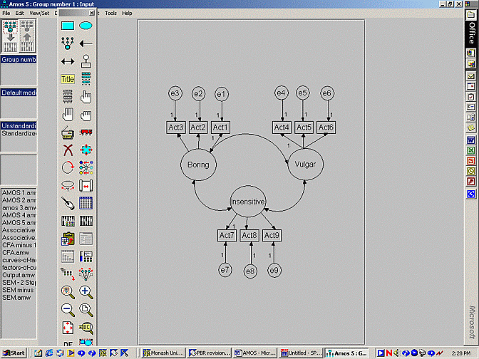
The hypothesised model is depicted in the worksheet above. The rectangles represent the variables that were actually measured - Acts 1 to 9. The circles represent the factors and error terms. The numbers that appear alongside each arrow represent coefficients. For example, if a 1 appears alongside an arrow, the model assumes the coefficient is 1. If no number appears alongside an arrow, the model will attempt to estimate this coefficient--a process that is outlined in another document.
Once this diagram is created, the process that needs to be followed to assess this model is straightforward. This document, hence, will primarily demonstrate the procedures that need to be followed to create these diagrams.
To activate AMOS:
To create a diagram that resembles the previous model, you will first need to depict the measured or observed variables--in this instance, Acts 1 to 9. The outcome of this step is presented below.
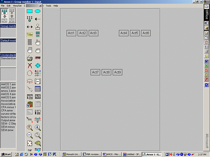
To create this diagram, you first need to ensure the tool box can be viewed. If the column of tools on the left of this screen is absent, select 'Show tools' from the 'Tools' menu. Then, to create a single rectangle:
To label this box:
To move this box to a suitable location:
To adjust the size of this rectangle:
To create eight more rectangles and thus represent the other measured variables:
You will then need to rename and reposition all the rectangles using the procedures outlined above.
If you commit an error, and would like to erase some object:
The next step is to present the factors - in this instance: boring, vulgar, and insensitive. The outcome of this step is presented below.
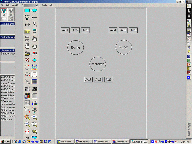
To create a single factor:
The next step is to create arrows that extend from the factors to the corresponding variables& otherwise, AMOS does not know which acts pertain to which factors. The outcome of this process is displayed below.
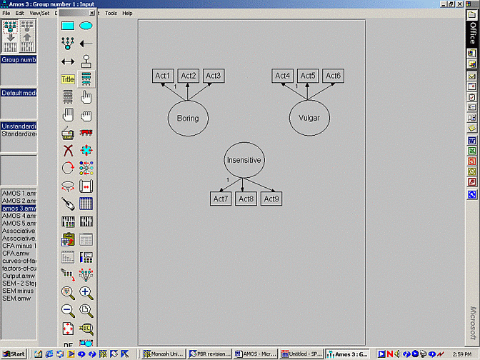
To create these arrows:
For each factor, one of the arrows needs to be designated as '1', as presented in the example above. For example, the arrow that links Act 1 to Boring could be designated as 1. This specification would indicate that:
Act 1 = 1 x Boring
rather than
Act 1 = B1 x Boring
As clarified in another document, this process imposes a scale on the factor& otherwise, scores on the factor could range from -1000 to 1000 or 1 to 10 or indeed anything. To stipulate this '1':
Occasionally, the box labelled 'Regression weight' will not appear. This problem arises when the arrow is too small, in which case the user has inadvertently selected a factor or variable. In this instance, the user should increase the distance between the factor and variable to extend the arrow.
In some models, the factors are assumed to be uncorrelated. In other instances, the factors are assumed to be correlated. To enable these correlations, you need to create a diagram that resembles the following illustration.
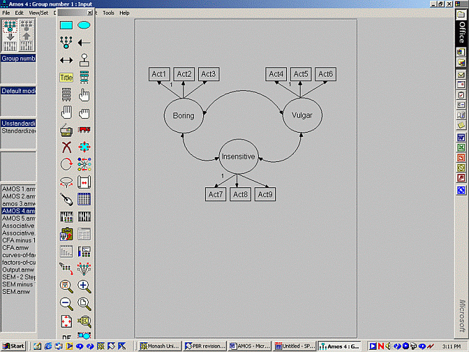
To create these double-headed arrows:
If you do not like the appearance of this double-headed arrow, you can adjust this procedure slightly. For example, you could click another factor first. Alternatively, you could begin the arrow at some other location within the factor.
Thus far, this model assumes that responses to each act depend only on the scores on corresponding factors. The effect of random sources of error has not been incorporated. For example, this model currently assumes that:
Act 9 = B9 x Insensitive
rather than
Act 9 = B9 x Insensitive + error
Clearly, these error terms need to be included. Responses to each act will never entirely depend on scores of the corresponding factors. Hence, the diagram will need to resemble the illustration below.
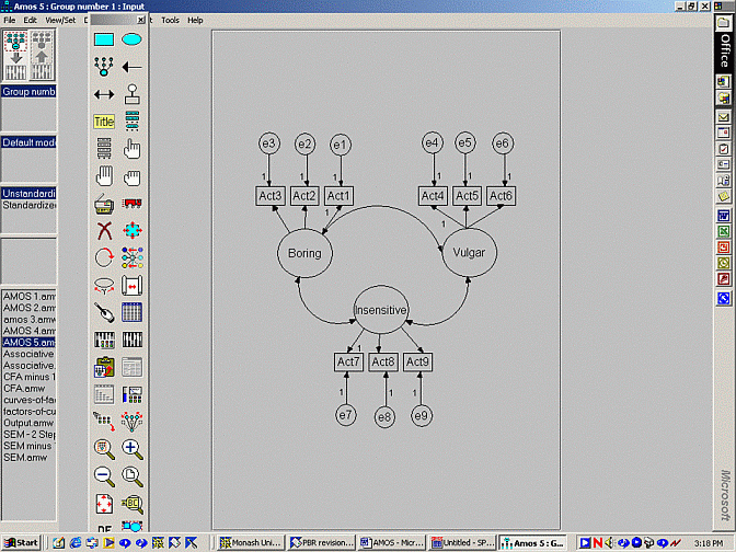
To create these error terms, the user can utilise all the principles outlined above. That is, errors are not measured and thus should appear as ovals, not rectangles. In short, to create these error terms:
The previous icons and processes are sufficient to create any diagram. Nevertheless, some of the other icons can accelerate the construction of these diagrams. To illustrate, consider the second icon from the top on the left-hand side. This icon can be utilised to construct a factor with several variables and error terms expediently. Specifically, the user merely needs to:
Likewise, the user might need to copy several objects at once. To achieve this goal:
Unfortunately, for some reason, this process cannot be utilised to copy arrows in the current version of AMOS.
Furthermore, some of the other icons can enhance the appearance of these diagrams. For example, suppose the measured variables are located above a factor. To rotate the factor, and thus position the variables to the left or right of some factor, activate the icon that appears below the cross. Then click the relevant factor.
In addition, sometimes the regression weights are obscured or overlap some other object. To move these numbers, activate the icon that resembles a circle above a Y. Then, click the mouse on the relevant arrow and drag in various directions.
Finally, in some instances, the drawing extends beyond the screen. To rectify this problem, you should locate an icon that displays a white piece of paper and 4 red arrows, usually towards the bottom end of the toolbox. When this icon is clicked, the diagram should appear within the boundaries of the worksheet. After the diagram is constructed and refined, the user should save this model, selecting 'Save' from the 'File' menu.
In short, the diagram represents a hypothesised model. To assess whether or not this model is consistent with the data, the user needs to specify the approach that AMOS should apply. For example, many different techniques can be utilised to assess this model. To stipulate the appropriate technique, the user should activate the icon that appears below the magic wand and above the clipboard on the left-hand side of the tool box. The dialogue box that appears enables the user to specify the precise approach that will be utilised to assess the model. For example, this box enables users to specify:
The output to present, such as standardised estimates, squared multiple correlations, tests of normality and outliers, indirect effects, modification indices and so forth.
Most of these issues are discussed in other documents. Nevertheless, in most instances, the default parameters are applicable. To assess the model, the user needs to activate the icon that appears adjacent to the previous icon that was utilised. This icon executes the analysis. Furthermore, to examine the output, the user needs to activate the icon that appears below the icon that executed the analysis.
Last Update: 6/2/2016