To illustrate the importance of interrupted time series, suppose the ABC news have decided to include canned laughter after each sentence that is uttered by the newsreader, ultimately to lighten the news and attract popularity. Now suppose a researcher wants to examine the number of individuals who watch the ABC news everyday before and after this intervention. The data are presented below. Each number represents the number of million who watched this program on a specific day.
Before intervention: 3.4, 5.6, 2.4, 6.5, 5.4, 1.2, 3.4... After intervention: 3.4, 6.5, 7.6, 6.8, 9.8. 7.8.
To ascertain whether or not this intervention was effective, the researcher might decide to compare the two sets of data--before and after the intervention--using an independent t-test. However, t-tests, and indeed most of the common statistical procedures, assume the data are independent.
In this instance, the assumption of independence is likely to be violated. If few individuals watch the news on one day, they might be more likely to watch the new on the next day--perhaps to override the feeling of ignorance they might experience. That is, the data point on one day might be negatively related to the data point on the previous day. Alternatively, if many individuals watch the news on one day, they might be more likely to watch the news on the next day--because they want to discover the upshot of some interesting story. Hence, the data point on one day might be positively related to the data point on the previous day.
Interrupted time series is a suite of techniques to examine how some event, such as an initiative, affects a pattern of data across time (McDowall, McCleary, Meidinger, & Hay, 1980). Typically, researchers apply a variant of the technique called ARIMA, or autorgressive moving average models (see Box & Jenkins, 1976;; Hoff, 1983), to examine these data. Rather than assume these data are independent, this approach comprises models that attempt to represent and control these dependencies.
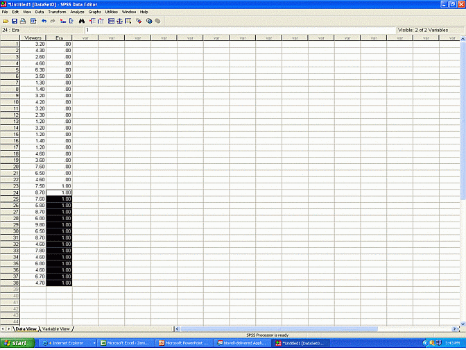
To learn ARIMA models, students should subject a hypothetical series of data, such as the number of individuals who watch the ABC news before and after some intervention, to SPSS. In particular, they should first construct a data sheet, as shown below, in which one column presents the data and another column specifies whether the data precedes or follows the intervention.

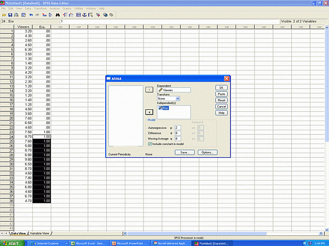
Second, they should select "Analyze", "Time series", and "ARIMA". The "Dependents" box refers to which column includes the data. The "Independents" box refers to which column specifies whether the data preceded or followed the intervention. Hence, in this instance, the researcher might assign the label "Viewers" to the "Dependents" box and the label "Era" to the "Independents" box.

Third, researchers should specify the number of autoregressive terms. To illustrate, suppose the researcher decides the number of individuals who watch the news one day is related to the number of individuals who watch the day before. In this instance, one autoregressive term should be included--implying that each data point is a function of the previous data point.
Suppose, instead, the researcher decides the number of individuals who watch the news one day is related to the number of individuals who watch the news during the previous two days They might argue that many stories culminate two daya later. Thus, if many individuals watch the news one day, they might be more likely to watch the news two days later. In this instance, two autoregressive terms should be included--implying that each data point is a function of the previous two data points.
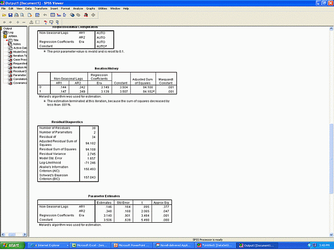
Fourth, researchers should press OK and then interpret the output. If the significancee or p value associated with the independent variable is significant, as shown in the table called "Parameter estimates", the researcher can conclude the intervention did affect the number of viewers, even after the autoregressive terms were controlled.

In the previous example, the number of viewers is likely to be a function of:
In this context, an error term does not refer to a mistake or blunder. Instead, the error term refers to all the other factors, apart from the intervention or autoregressive terms, that could affect the number of viewers--perhaps the weather, other TV programs that day, special events such as the superbowl, and so forth.
Sometimes, the error term on one day, sometimes called a random shock, depends on the error term on the previous day. For example, perhaps a unique event that raises the number of viewers on one day, such as the superbowl, will tend to reduce the number of viewers on the next day, perhaps because of intoxication. In this instance, the researcher will tend to include another parameter, called a moving average.
Similarly, the error term on one day can depend on the error terms of the two previous days. In this instance, the researcher will tend two include two moving averages in the appropriate box.
This technique also assumes the series of data are stationary--that is, roughly stable across time, apart from the impact of any interventions. More precisely, the average value, as well as the variability and distribution of these values, should be roughly the same across the entire range.
Sometimes, the difference between two consecutive data points, and not the data points themselves, are stationary. For TV programs that are becoming increasingly popular over time, for example, the increase in viewers each day, not the number of viewers each day, might be stationary and stable.
In these instances, researchers should ensure that SPSS examines the difference between two consecutive values, not the actual values. In particular, to achieve this goal, they should assign a 1 to the box labelled "Differences".
Box, G. E. P., & Jenkins, G. M. (1976). Time series analysis: Forecasting and control. San Francisco: Holden-Day.
Hoff, J. C. (1983). A practical guide to Box-Jenkins forecasting. London: Lifetime Learning Publications.
McDowall, D., McCleary, R., Meidinger, E. E., & Hay, R. A. (1980). Interrupted time series analysis. Beverly Hills, CA: Sage Publications.
Melard, G. (1984). A fast algorithm for the exact likelihood of autoregressive-moving average models. Applied Statistics, 33, 104-119.
Pankratz, A. (1983). Forecasting with univariate Box-Jenkins models: Concepts and cases. New York: Wiley.
Vandaele, W. (1983). Applied time series and Box-Jenkins models. New York: Academic Press.
Last Update: 6/1/2016